Fast MRI · Multi-View
Cross-Plane Consistency for Accelerated MRI
Radiologists read a volume by switching between sagittal, axial and coronal planes — but accelerated reconstructions are rarely equally good in all three. VSSR cascades three view-specialized 2D networks to refine the volume plane by plane, reaching better fidelity than a 3D network at a quarter of its memory.
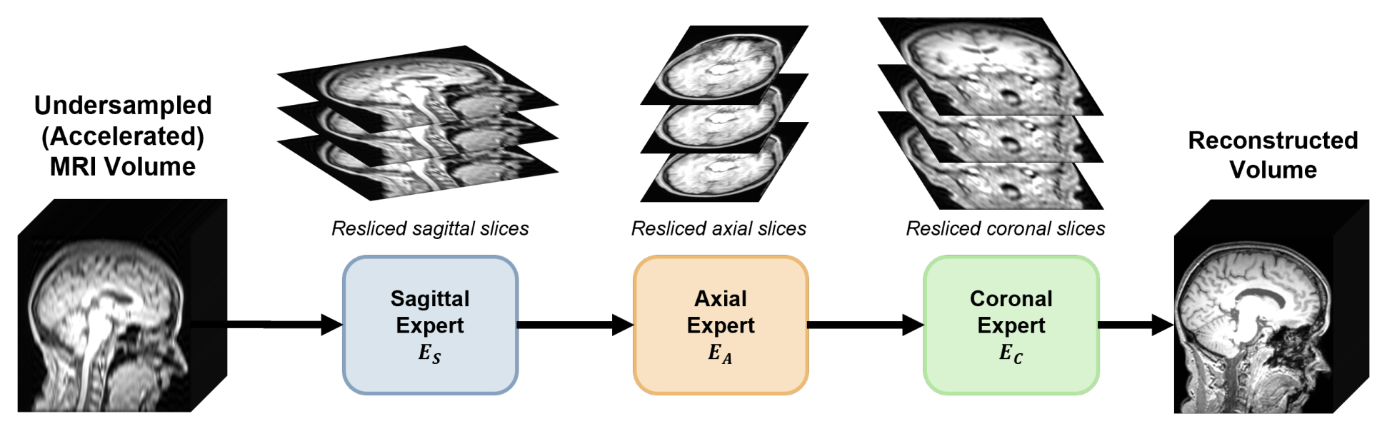
A volume is read in three planes, not one
Accelerating an MRI acquisition by reducing phase-encoding coverage cuts scan time, but it degrades the reconstruction through aliasing and loss of effective resolution. Deep learning recovers much of that quality — yet methods are usually developed and judged from a purely algorithmic standpoint, on the plane they happen to be trained on.
That is not how the images are used. In practice radiologists interrogate 3D anatomy by scrolling through slices and switching between sagittal, axial and coronal views. Quality that holds up in one plane and collapses in another is a clinical problem, not a cosmetic one: view-dependent artifacts also hinder downstream tasks such as segmentation and quantitative assessment.
We therefore address a specific, deliberately practical setting — post-reconstruction volumetric refinement. Given a reconstructed magnitude volume from an accelerated acquisition, whatever produced it (a vendor pipeline, any reconstruction method), improve its cross-plane consistency and fidelity without access to raw k-space and without touching data-consistency operations.
Why 2D and 3D both fall short
Learning-based approaches split into two camps. 3D networks capture rich volumetric context, but their memory footprint forces patch-based training and inference or reduced resolution, which complicates whole-volume deployment and introduces boundary effects. 2D networks are memory-efficient and operate on full slices, but treat those slices independently — nothing in them enforces inter-slice or cross-plane consistency.
Intermediate strategies exist. 2.5D methods feed several adjacent slices from a single orientation to add limited volumetric context, and early multi-view CNNs combined predictions from orthogonal orientations. But these process each plane independently, or fuse the views exactly once. None of them lets information propagate across planes, where a later view can correct what an earlier one left behind.
Multi-stage cascades, by contrast, have proven effective for progressive refinement in MRI recovery, each stage correcting the residual errors of the last. That is the principle we bring to the multi-view problem.
Our approach: View-Specialized Sequential Refinement
VSSR is a cascade of three 2D expert networks, each specialized to one anatomical plane. Starting from the accelerated volume V₀, the sagittal expert produces V₁; the axial expert refines that into V₂; the coronal expert produces the final output V₃:
Every expert is trained only on its designated plane, which encourages view-specific feature learning. Because the experts run in sequence rather than in parallel, later stages correct residual errors left by earlier ones, and information propagates across planes — so cross-plane consistency emerges without an explicit 3D consistency term, and without ever loading a volume into a 3D network.
The design is backbone-agnostic: any 2D slice-to-slice restoration network can serve as an expert. Here each expert is a Swin-UNet of roughly 30M parameters, chosen for its strong 2D performance and favourable memory profile.
Progressive training
The experts are trained one after another, each on the output distribution the preceding stages actually produce — which removes the train–test mismatch a naively assembled cascade would suffer:
- Phase 1 — the sagittal expert ES is trained on sagittal slices of V₀ with an ℓ₁ loss against the fully sampled reference.
- Phase 2 — ES is applied across the training set to generate V₁, and the axial expert EA is trained on axial slices of V₁, correcting what the sagittal stage left behind.
- Phase 3 — the cascade EA(ES(·)) generates V₂, and the coronal expert EC is trained on coronal slices of it, refining the output of both preceding experts.
Training uses AdamW (learning rate 10⁻⁴ with cosine annealing, batch size 16) on a single NVIDIA RTX 3090, for 60, 40 and 50 epochs respectively. Implementation is in PyTorch 2.0.0 with MONAI 1.3.0 and SimpleITK 2.3.0. Code and pretrained models: github.com/MR-Nazarov/VSSR.
Results on the IXI benchmark
Retrospective evaluation uses 581 T1-weighted brain volumes (256×256×128) from the IXI dataset, split 407/87/87 for training, validation and test. Acceleration is simulated by truncating k-space along a single phase-encoding direction, keeping the central 25% of lines for 4× and 12.5% for 8× — a rectangular truncation that matches the direction-dependent resolution loss of our real accelerated acquisition.
VSSR is compared against a 3D U-Net (21M parameters, ~8 GB peak inference memory), a single-view sagittal Swin-UNet (30M, ~2 GB) and a 2D ensemble that averages three independently trained view-specific Swin-UNets.
| Method | PSNR 4× | SSIM 4× | PSNR 8× | SSIM 8× |
|---|---|---|---|---|
| Zero-filling | 31.52 | 0.928 | 28.08 | 0.825 |
| 3D U-Net | 34.49 | 0.966 | 31.02 | 0.921 |
| Sagittal Swin-UNet | 34.45 | 0.966 | 30.70 | 0.917 |
| 2D ensemble | 34.50 | 0.965 | 31.01 | 0.919 |
| VSSR (ours) | 34.95 | 0.969 | 31.28 | 0.926 |
Volume-level PSNR (dB) and SSIM on the IXI test set (87 volumes). VSSR is best at both acceleration factors, while needing 2 GB of peak inference memory against the 3D U-Net's 8 GB. All differences are statistically significant (Wilcoxon signed-rank, p < 0.001).
That VSSR also beats the 2D ensemble matters: both use the same three view-specific backbones, so the gain comes from sequencing them rather than from merely combining independent view-wise predictions.
Consistency across planes
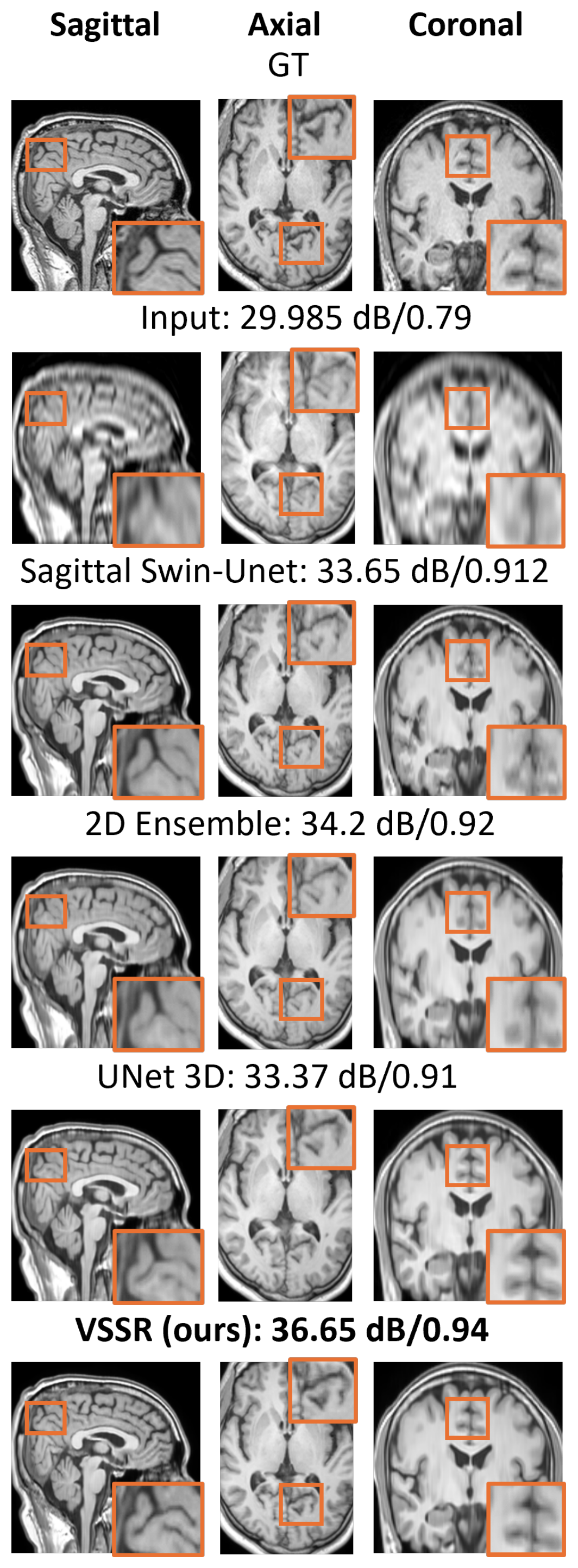
Per-view metrics at 8× acceleration show the failure mode the method targets. A single-view expert is excellent in its trained plane and noticeably worse elsewhere — the sagittal Swin-UNet leads in sagittal view at 34.45 dB, then drops to 31.65 dB coronally. The ensemble evens this out but still varies. VSSR gives the highest mean across the three planes and the most balanced profile.
| Method (8×) | Sagittal | Axial | Coronal | Mean |
|---|---|---|---|---|
| PSNR (dB) | ||||
| Zero-filling | 29.00 | 29.24 | 32.97 | 30.40 |
| 3D U-Net | 31.84 | 34.03 | 35.61 | 33.83 |
| Sagittal Swin-UNet | 34.45 | 35.54 | 31.65 | 33.88 |
| 2D ensemble | 31.89 | 34.67 | 35.72 | 34.09 |
| VSSR (ours) | 32.18 | 35.10 | 35.92 | 34.40 |
| SSIM | ||||
| Zero-filling | 0.799 | 0.849 | 0.827 | 0.825 |
| 3D U-Net | 0.899 | 0.914 | 0.910 | 0.907 |
| Sagittal Swin-UNet | 0.911 | 0.906 | 0.894 | 0.904 |
| 2D ensemble | 0.897 | 0.913 | 0.908 | 0.906 |
| VSSR (ours) | 0.905 | 0.920 | 0.915 | 0.914 |
Per-view quality at 8× acceleration. Mean values are averaged over the three anatomical views.
The same effect is plain to the eye. Below, one test case at 8× acceleration is shown in all three planes at once — the comparison a radiologist would effectively make when scrolling through a study. The accelerated input has lost fine cortical detail in every view. The sagittal Swin-UNet restores its own plane convincingly but leaves the coronal view smeared, the failure its 31.65 dB coronal score records. The 2D ensemble and the 3D U-Net land in between. VSSR is the only row where the magnified insets hold up in all three planes at once.
Validation on real accelerated scans
Retrospective undersampling does not reproduce scanner-specific noise or vendor reconstruction behaviour, so the method was also validated prospectively. Healthy volunteers were scanned at Sheba Medical Center on a 1.5T Philips Ingenia (TR 7.5 ms, TE 3.4 ms). The fully sampled reference was acquired at 240×240×240 with isotropic 1 mm³ resolution in 4.58 minutes; the accelerated T1-weighted volume reduced the anterior–posterior phase-encoding matrix to 240×60×240 — a genuine 4× acceleration — in 1.13 minutes. Both were reconstructed by the scanner's own Philips compressed-sensing pipeline, with the fully sampled reconstruction rigidly registered to the accelerated one for evaluation.
| Method (real 4×) | 3D PSNR | 3D SSIM | Mean 2D PSNR | Mean 2D SSIM |
|---|---|---|---|---|
| Accelerated input | 13.99 | 0.711 | 17.45 | 0.710 |
| 3D U-Net | 27.83 | 0.888 | 30.81 | 0.872 |
| Sagittal Swin-UNet | 29.72 | 0.922 | 33.63 | 0.910 |
| VSSR (ours) | 30.98 | 0.935 | 35.23 | 0.922 |
Prospectively acquired 4× accelerated clinical volumes, after fine-tuning on 15 cases. Mean 2D metrics are averaged across the three anatomical views.
VSSR improves over the 2D baseline by 1.60 dB in mean cross-plane PSNR and over the 3D U-Net by more still — evidence that the gains survive the move from simulated undersampling to a real vendor pipeline, with its own scanner noise and reconstruction behaviour.
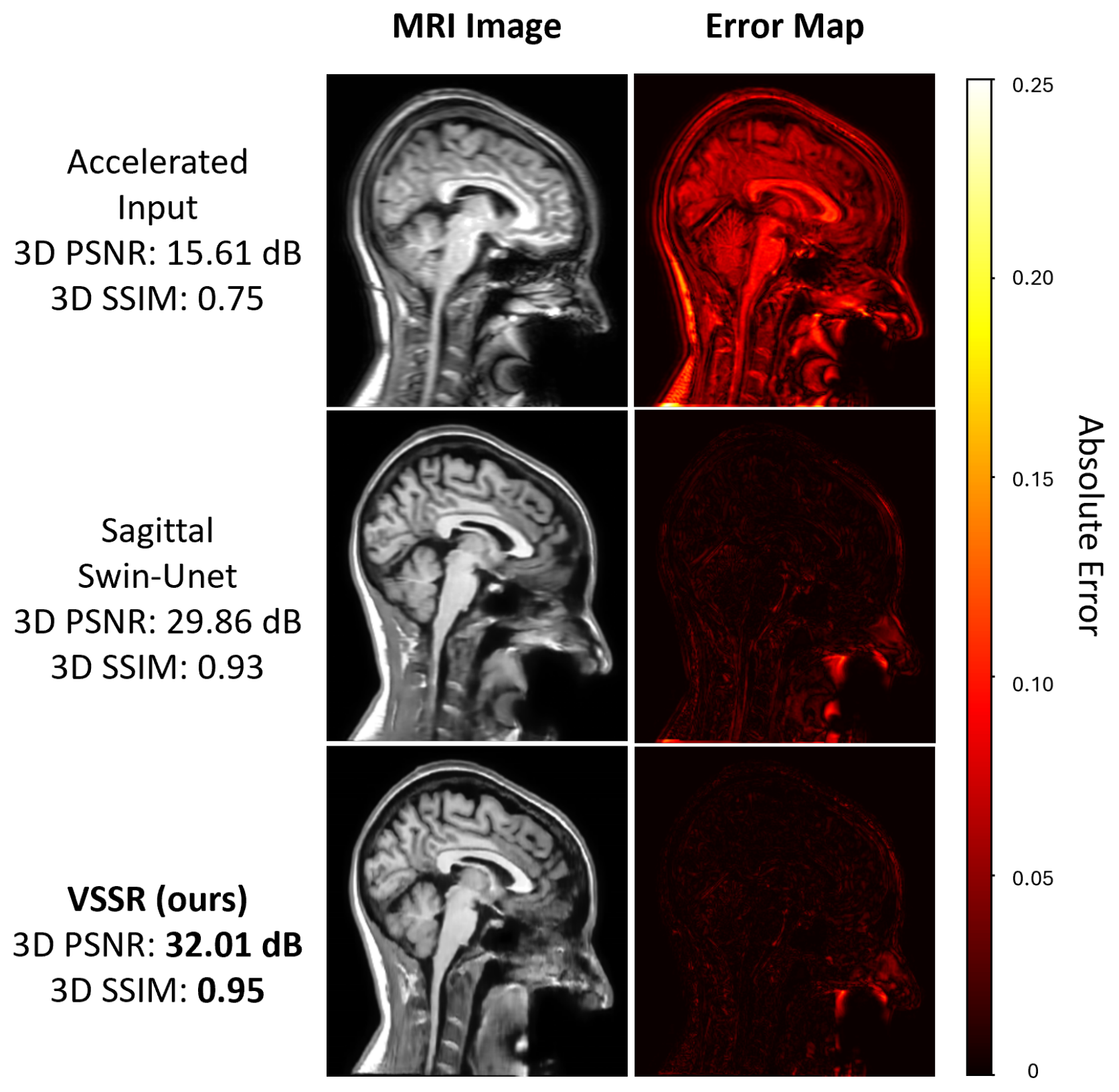
The error maps make the margin concrete. Below, a representative case is shown against the fully sampled reference: the accelerated input carries error across the whole head, brightest along the skull, the corpus callosum and the cervical spine. The sagittal Swin-UNet removes most of it. VSSR removes more still, and what remains is confined to thin edges rather than spread through the parenchyma — 32.01 dB against the baseline's 29.86 dB on this case.
The order of the cascade matters
An ablation at 8× acceleration tests both halves of the design: whether the stages actually accumulate, and whether their order is arbitrary. Both answers are informative. Refinement is cumulative — sagittal alone reaches 30.70 dB, adding the axial expert 30.74 dB, and the full three-stage cascade 31.28 dB. And the ordering is emphatically not arbitrary.
| Configuration (8×) | 3D PSNR | 3D SSIM | Mean 2D PSNR | Mean 2D SSIM |
|---|---|---|---|---|
| S→A→C path (proposed) | ||||
| Stage 1: S | 30.70 | 0.917 | 33.88 | 0.904 |
| Stage 2: S→A | 30.74 | 0.918 | 33.92 | 0.905 |
| Stage 3: S→A→C | 31.28 | 0.926 | 34.40 | 0.914 |
| Alternative orders | ||||
| A→S→C | 30.08 | 0.908 | 33.13 | 0.897 |
| C→A→S | 30.50 | 0.912 | 33.51 | 0.901 |
Ablation at 8× acceleration. Mean 2D metrics are averaged across views; every configuration uses identical backbones.
The proposed S→A→C ordering beats A→S→C by 1.20 dB with the same networks. We attribute the sensitivity to the direction-dependent degradation that phase-encoding matrix reduction produces: the resulting blur manifests differently in each plane, and the first stage in the cascade sets the error distribution every later expert has to work with. The working hypothesis is that the best order is tied to the acceleration direction — which axis loses the most high-frequency content — and a systematic study across phase-encoding directions is left for future work.
Summary & outlook
VSSR lets efficient 2D slice-based networks deliver volumetric fidelity and cross-plane consistency that neither single-view 2D processing nor simple multi-view averaging achieves — and it does so at 2 GB of peak inference memory against 8 GB for a 3D U-Net. That efficiency is the practical point: many MRI pipelines favour 2D models precisely because of memory limits and the scarcity of large-scale 3D training data.
Because the method operates on reconstructed magnitude volumes, it drops in behind an existing clinical pipeline without access to raw k-space and without altering data-consistency operations. Future work will evaluate additional 2D expert backbones, explore joint end-to-end training of the full cascade, and extend the approach to other anatomies, modalities and multi-contrast settings — including the multi-contrast line of work alongside it.
Ethics. Retrospective experiments use the IXI dataset, available under the Creative Commons CC BY-SA 3.0 licence. The clinical validation cases were handled in line with the principles of the Declaration of Helsinki, with approval granted by the IRB of Sheba Medical Center. No funding was received for this study, and the authors have no relevant financial or non-financial interests to disclose.
References
- Lustig, M., Donoho, D. and Pauly, J.M., 2007. Sparse MRI: the application of compressed sensing for rapid MR imaging. Magnetic Resonance in Medicine, 58(6), pp.1182–1195.
- Fan, C.-M., Liu, T.-J. and Liu, K.-H., 2022. SUNet: Swin Transformer UNet for image denoising. In IEEE International Symposium on Circuits and Systems (ISCAS), pp.2333–2337.
- Schlemper, J., Caballero, J., Hajnal, J.V., Price, A.N. and Rueckert, D., 2017. A deep cascade of convolutional neural networks for dynamic MR image reconstruction. IEEE Transactions on Medical Imaging, 37(2), pp.491–503.
- Zhang, Y., Liao, Q., Ding, L. and Zhang, J., 2022. Bridging 2D and 3D segmentation networks for computation-efficient volumetric medical image segmentation: an empirical study of 2.5D solutions. Computerized Medical Imaging and Graphics, 99, p.102088.
- Dolz, J., Desrosiers, C. and Ben Ayed, I., 2018. 3D fully convolutional networks for subcortical segmentation in MRI: a large-scale study. NeuroImage, 170, pp.456–470.
- Feng, C.-M., Fu, H., Yuan, S. and Xu, Y., 2021. Multi-contrast MRI super-resolution via a multi-stage integration network. In MICCAI 2021, pp.140–149.
- Imperial College London, 2008. Information eXtraction from Images (IXI) Dataset. brain-development.org/ixi-dataset.
- Knoll, F., Zbontar, J., Sriram, A., Muckley, M.J., Bruno, M., Defazio, A. et al., 2020. fastMRI: a publicly available raw k-space and DICOM dataset of knee images for accelerated MR image reconstruction using machine learning. Radiology: Artificial Intelligence, 2(1), e190007.
Content on this page is drawn from “Post-Reconstruction Volumetric Refinement for Accelerated MRI via Cross-Plane Consistency” (A. Nazarov, N. Kiryati, D. Roizen, G. Greenberg, A. Mayer).