Project
Ultra-Fast DTI
White matter tractography from a four-minute diffusion scan instead of nineteen — a collaborative neural framework that denoises low-angular-resolution diffusion data and segments the tracts in a single pipeline.
Why diffusion tractography is slow
Diffusion tensor tractography is the way we map white matter in vivo — the wiring of the brain, traced non-invasively. It is indispensable for neurosurgical planning. It is also slow at both ends: a long acquisition, followed by tedious manual work to produce usable tracts.
The acquisition cost has a simple structure. Scan time is proportional to the number of diffusion-encoding gradient directions (NDGD) — each direction is another set of images to acquire. Fitting the tensor model at all requires a minimum of six non-collinear gradient-weighted scans plus one reference, but nobody scans at six: raising the NDGD improves signal-to-noise, makes the fitted tensor more robust, and samples diffusion at a higher angular resolution, which yields visibly better tractography. So protocols climb to 64 directions and beyond, and the patient lies in the magnet for 19 minutes.
Then the second cost arrives. Turning DTI maps into subject-specific tracts still means seeding, drawing, and manually removing outliers by hand.
Two problems, solved separately
Both halves have had attention — but in isolation, and with gaps.
On the acceleration side, SuperDTI learns to map DWI images straight to DTI maps, bypassing tensor fitting, and claims quality tractography from as few as six directions — but validates only on synthesised low-direction data, and scores tractography by counting reconstructed fibres rather than measuring spatial overlap. DeepDTI denoises six DWI volumes against a ground truth synthesised from additional data, claiming a 3.5–4× speed-up. SDnDTI removes the need for high-SNR training data through self-supervision. Neither provides tract-level validation.
On the segmentation side, TractSeg segments tracts directly from fibre orientation distribution peaks, and multi-sequence CNN workflows have been proposed for joint registration and segmentation of tracts. But this work assumes high-quality input: at least 64 directions, and often far more.
Our goal: optimise the whole workflow
We treat acquisition and segmentation as one problem. The framework takes the Diffusion Encoded Colour (DEC) map computed from a low-direction DWI acquisition, enhances it with a denoising network, and hands the result to a segmentation network that produces the tracts — collapsing both pain points into a single automatic pass.
The contributions are three:
- A fully automatic collaborative framework that turns DEC maps from low-direction DWI into high-quality tract segmentations.
- A novel spherical k-means method for selecting an approximately uniform subset of gradient directions out of a high-direction set.
- A novel diffusion loss for training the DEC map denoiser.
Which 16 directions? Spherical k-means
To train a network to work at low NDGD you need low-NDGD data. There are two ways to get it, and they trade off against each other. Acquire real pairs of low- and high-direction scans, and you learn a realistic mapping — but every training case costs another scanning session. Synthesise the low-direction set from high-direction data, and it scales freely — but interpolation-based synthesis produces smoothed maps that do not look like a real low-direction acquisition at all.
Our answer sidesteps interpolation. Rather than blending the full angular information into a smaller set, we select an actual subset of gradient directions that offers pseudo-optimal angular coverage. The directions live on the unit sphere, so we cluster them there: spherical k-means with k set to the desired NDGD, then pick from each cluster the direction closest to its centroid.
The distance metric is the point. Cosine distance measures angular dissimilarity directly, which is exactly what "spread these directions evenly over a sphere" means — an L1 or L2 norm would not.
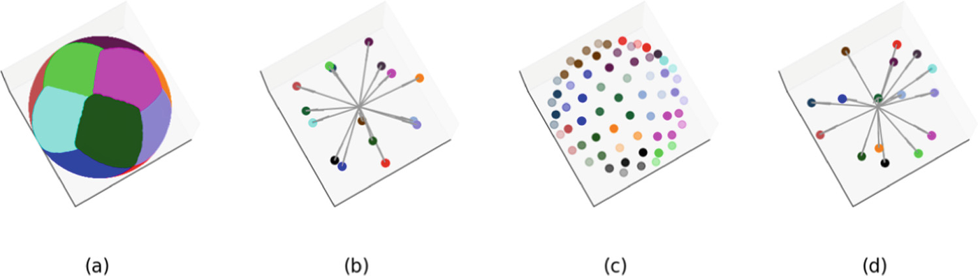
Selected subsets look like real low-direction acquisitions because they are real acquisitions — just fewer of them. Interpolated ones, by comparison, are visibly over-smoothed, which makes them a misleading proxy to train or validate against.
A loss that speaks diffusion
A generic image loss treats a DEC map as a picture. It is not a picture — it is a physical quantity in disguise. Each voxel's RGB value is the fractional anisotropy multiplied by the absolute principal diffusion direction:
Both quantities are recoverable from the RGB map — which means the loss can supervise them separately, each in the metric it deserves. FA is a magnitude, so it gets an L1 distance. PDD is a unit vector field, so it gets a cosine distance, which measures angular error directly. That matters because the PDD is what determines which way a tract runs: get the angle wrong and the tractography goes somewhere else, however pretty the image looks.
One wrinkle needs handling: where FA is degenerate the division by FA is undefined. This affects roughly 0.3% of brain voxels, which are assigned an arbitrary PDD of (1, 0, 0) as a numerical workaround.
Experiments
Two datasets, doing different jobs
The HCP dataset supplies scale and angular resolution: 105 cases at 270 directions, split 74 training / 11 validation / 20 test, with bilateral motor tract ground truth generated following the TractSeg protocol. Spherical k-means reduces each case to a 16-direction subset.
The clinical dataset supplies reality: 10 prospective cases acquired at Sheba Medical Center on a Philips 1.5T Ingenia, each scanned twice — once at 16 directions and once at 64, so the low-direction input is a genuine fast acquisition rather than a simulation of one. Tensors, DEC and FA maps were computed with DIPY; the motor tract ground truth came from Contrack probabilistic tractography; cases were aligned to MNI space with FSL-FLIRT and brain-masked with ANTsPyNet. Evaluation is 5-fold cross-validation.
Training the pair together — where memory allows
For the DnCNN3D → Unet-3D pipeline the two networks are trained as a cascade under a joint loss: the denoising term contributes 0.6, the segmentation Dice term 0.4, both brain-masked and normalised to [0, 1] so they are comparable. This is what makes the framework collaborative rather than merely sequential — the denoiser is partly optimised for what the segmenter needs. Clinical training starts from the HCP-trained weights by transfer learning.
For DnCNN3D → Swin-UNETR joint training was not possible: Swin-UNETR's memory demands ruled it out. Instead the DnCNN3D from the previous scenario is frozen, training data is pushed through it, and Swin-UNETR is trained on the output with self-supervised pre-training. Fold partitions were kept identical across both networks so that each was tested only on cases it had never seen.
Results
Map quality
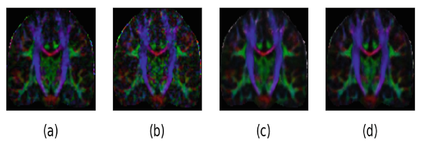
On the real 16-direction clinical scans, denoising moves both map-quality indices substantially — and the two losses land in a near dead heat.
| Metric (clinical, 16 directions) | Before denoising | DnCNN3D, L1 loss | DnCNN3D, diffusion loss |
|---|---|---|---|
| DEC map SSIM ↑ | 0.560 | 0.680 | 0.681 |
| FA map L1 distance ↓ | 0.075 | 0.051 | 0.052 |
Tract quality — where the pipeline choice shows
The tract Dice is the number that matters, and it separates the two segmentation architectures sharply.
| Pipeline (clinical, 5-fold) | Input | Bilateral motor tract Dice ↑ |
|---|---|---|
| Unet-3D, no denoising | 16 directions | 0.42 |
| DnCNN3D → Unet-3D | 16 directions | 0.44 |
| Swin-UNETR, no denoising | 16 directions | 0.59 |
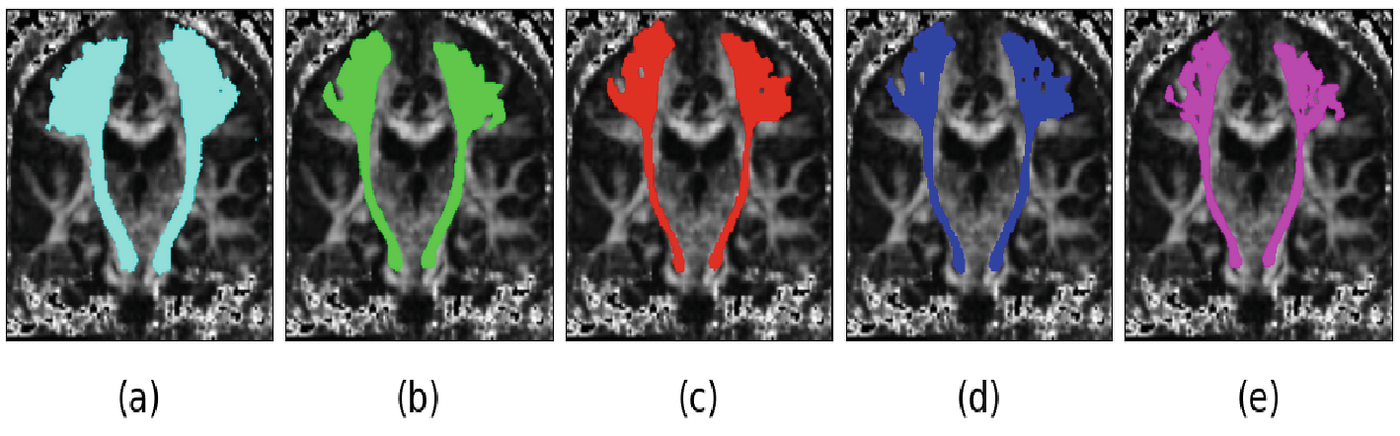
| DnCNN3D → Swin-UNETR (proposed) | 16 directions | 0.70 |
| Swin-UNETR on a real 64-direction scan | 64 directions | 0.74 |
The proposed pipeline reaches 0.70 from a four-minute scan, against 0.74 from the full nineteen-minute acquisition — most of the tract quality, at roughly a fifth of the scan time. Denoising is doing real work here: the same Swin-UNETR without it drops to 0.59.
Not every pairing benefits equally. Unet-3D barely moves (0.42 → 0.44) while Swin-UNETR gains eleven points, which suggests some denoising–segmentation pairs are genuinely more synergistic than others rather than denoising being uniformly good.
The finding that only real data could reveal
On HCP — where the 16-direction data is simulated by subset selection — Swin-UNETR's Dice was the best on offer but appeared essentially insensitive to prior denoising. On the clinical data, where the 16-direction scans are real, the same architecture swings from 0.59 to 0.70 depending on whether it was denoised first.
This is the strongest argument for the dual-acquisition dataset, and it generalises past this paper: validating an acceleration method on synthetically decimated data can hide the very effect the method exists to produce. Across the experiments the diffusion loss slightly outperformed L1 in almost every case — a real but modest edge, not the headline.
Discussion & outlook
The framework generates high-quality bilateral motor tracts from 16 gradient directions acquired on a 1.5T magnet in four minutes, down from nineteen, with tract Dice approaching what a full 64-direction scan delivers. Acquisition and post-processing collapse into one automatic pass.
The clearest application is intra-operative navigation, where both the magnetic field and the available time are constrained — exactly the regime where a fast, low-field, automatic pipeline is worth the most. On 3T diagnostic scanners the same methods should permit even faster acquisitions, improving both patient experience and scanner throughput.
The honest limits: 10 clinical cases is a small cohort, and validation covers the bilateral motor tracts rather than the full tract atlas. Future work is extensive validation on larger clinical datasets, and finding the NDGD that best balances scan time against image quality — a number that will likely differ between diagnostic imaging and neurosurgical planning.
Published at CDMRI 2023 (Computational Diffusion MRI, MICCAI workshop), Lecture Notes in Computer Science, vol. 14328, pp. 118–128, Springer. doi:10.1007/978-3-031-47292-3_11
References
- O. Leshem, N. Kiryati, M. Green, I. Nelkenbaum, D. Roizen, and A. Mayer, "Fast Acquisition for Diffusion Tensor Tractography," in M. Karaman et al. (Eds.), Computational Diffusion MRI (CDMRI) 2023, LNCS vol. 14328, pp. 118–128, Springer, 2023.
- P. J. Basser, J. Mattiello, and D. LeBihan, "MR diffusion tensor spectroscopy and imaging," Biophysical Journal, vol. 66, no. 1, pp. 259–267, 1994.
- S. Pajevic and C. Pierpaoli, "Color schemes to represent the orientation of anisotropic tissues from diffusion tensor data: application to white matter fiber tract mapping in the human brain," Magnetic Resonance in Medicine, vol. 42, no. 3, pp. 526–540, 1999.
- I. S. Dhillon and D. S. Modha, "Concept decompositions for large sparse text data using clustering," Machine Learning, vol. 42, pp. 143–175, 2001.
- D. Liu, W. Wang, X. Wang, C. Wang, J. Pei, and W. Chen, "Poststack seismic data denoising based on 3-D convolutional neural network," IEEE Transactions on Geoscience and Remote Sensing, vol. 58, no. 3, pp. 1598–1629, 2019.
- Y. Tang, et al., "Self-supervised pre-training of Swin transformers for 3D medical image analysis," IEEE/CVF Conference on Computer Vision and Pattern Recognition (CVPR), pp. 20730–20740, 2022.
- Ö. Çiçek, A. Abdulkadir, S. S. Lienkamp, T. Brox, and O. Ronneberger, "3D U-Net: learning dense volumetric segmentation from sparse annotation," MICCAI 2016, LNCS vol. 9901, pp. 424–432, Springer.
- J. Wasserthal, P. Neher, and K. H. Maier-Hein, "TractSeg — fast and accurate white matter tract segmentation," NeuroImage, vol. 183, pp. 239–253, 2018.
- H. Li, et al., "SuperDTI: ultrafast DTI and fiber tractography with deep learning," Magnetic Resonance in Medicine, vol. 86, no. 6, pp. 3334–3347, 2021.
- Q. Tian, et al., "DeepDTI: high-fidelity six-direction diffusion tensor imaging using deep learning," NeuroImage, vol. 219, 117017, 2020.
- Q. Tian, et al., "SDnDTI: self-supervised deep learning-based denoising for diffusion tensor MRI," NeuroImage, vol. 253, 119033, 2022.
- A. J. Sherbondy, R. F. Dougherty, M. Ben-Shachar, S. Napel, and B. A. Wandell, "ConTrack: finding the most likely pathways between brain regions using diffusion tractography," Journal of Vision, vol. 8, no. 9, 15, 2008.
- E. Garyfallidis, et al., "DIPY, a library for the analysis of diffusion MRI data," Frontiers in Neuroinformatics, vol. 8, 8, 2014.
- N. Barzilay, I. Nelkenbaum, E. Konen, N. Kiryati, and A. Mayer, "Neural registration and segmentation of white matter tracts in multi-modal brain MRI," ECCV 2022 Workshops, LNCS vol. 13803, Springer, 2022.
- D. C. Van Essen, et al., "The human connectome project: a data acquisition perspective," NeuroImage, vol. 62, no. 4, pp. 2222–2231, 2012.