Project
PET MIP AI
Segmenting tumours directly on the rotating projections radiologists actually read — matching full 3D accuracy while cutting training time four-fold and compute by over two orders of magnitude.
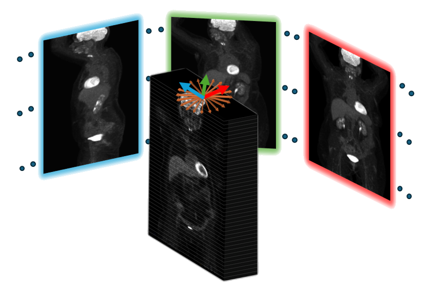
How radiologists actually read a PET scan
PET/CT is the gold standard for finding tumours, and for spotting metastatic disease anywhere in the body. But a whole-body PET volume is a lot of data, and radiologists do not start by scrolling through it slice by slice.
They start with a rotating Maximum Intensity Projection. A MIP takes the brightest value along each line of sight and collapses the volume into a single 2D image; spin it through a series of yaw angles and you get a short loop that shows every region of high tracer uptake in the body at once. Reviewing that rotating loop before reading the patient history is a deliberate part of the workflow — it favours an unbiased, "gestalt" read of the case. Only then does the radiologist confirm findings in the volumetric slices.
That confirmation step is where the time goes, especially in metastatic cases where lesions are scattered. Marking suspicious regions automatically on the rotating MIP would point the reader straight at what matters.
But that is not where the models look
Automated PET analysis has gone the other way. Most deep learning models treat PET as a stack of slices and segment the 3D volume, ignoring the projections entirely. Where MIPs do appear, they are usually a supporting actor: a detector run over multi-orientation MIPs to flag physiological uptake, an Xception model on multi-angle MIPs for breast cancer classification, sagittal and coronal MIPs used as a gate to suppress false positives, or MIP-derived features feeding a survival model.
A few studies have gone further — showing that MIP representations can improve 3D PET/CT segmentation, or reconstructing volumetric segmentations back from 2D MIPs. But direct segmentation on MIPs, evaluated on its own terms, has largely gone unexamined.
The case for training on them is not just philosophical. MIPs are a drastically compact representation: 16 views carry roughly 4% of the volumetric information while keeping the lesion detail that matters. That compactness means smaller memory footprints, ordinary hardware, faster iteration, and lightweight models that suit real-time clinical use. And aligning the model's input domain with the radiologist's diagnostic perspective means it learns clinically relevant features by construction.
Our goal: train where the radiologist looks
The conventional pipeline segments the 3D volume and then projects the result to a MIP if a projection is needed. We invert that: project first, segment second. The model never sees a volume.
Building the projections
Each MIP is formed by rotating the volume about the superior–inferior (yaw) axis and taking the maximum along the anterior–posterior depth axis:
Data
Experiments use the open-source autoPET 2022 dataset: 1,014 PET/CT scans from 900 patients, each with a 3D PET scan, a CT scan and a tumour segmentation map. PET values were standardised to SUV units. We use PET MIPs rather than CT MIPs, since PET is what whole-body tumour assessment is based on — and it makes the comparison against 3D PET segmentation a fair one.
| Class | Negative (healthy) | Lymphoma | Melanoma | Lung cancer |
|---|---|---|---|---|
| Cases | 513 | 145 | 188 | 168 |
15% of the data was set aside as an independent test set; the remaining 85% drove 5-fold cross-validation, with the class distribution preserved across every split.
The occlusion problem — and how we fix the labels
Projecting a 3D annotation onto a MIP creates a subtle trap. A MIP keeps only the brightest value along each ray. The brain, heart and kidneys take up FDG avidly, so when a lesion happens to line up behind one of them at a given angle, the organ wins the projection and the tumour is simply not visible in that view.
The annotation, however, gets projected regardless. The result is a label that marks a tumour on a pixel where no tumour is visible — teaching the network to hallucinate lesions inside bright organs, and producing false positives.
Because projection is traceable — every MIP pixel can be mapped back to the voxel that produced it — the fix is tractable:
- Occlusion detection. For each labelled tumour in a MIP, check that at least 75% of its pixels genuinely originated from tumour voxels in the 3D data.
- Annotation splitting. If it falls below 75%, split the label and keep only the pixels confirmed to come from the tumour.
- Low-contrast filtering. Remove leftover fragments of tumours whose contrast is so low they would be undetectable by eye anyway.
The principle is that a tumour occluded in a projection is one a radiologist could not see either, so the label should not claim otherwise. The correction is also surgical rather than destructive: only 0.57% of tumours were dropped from all MIPs, accounting for just 0.09% of the original volumetric tumour volume. Both the original projected labels (OR-MIPs) and the occlusion-corrected ones (OC-MIPs) are carried through the experiments.
Results: MIPs versus 3D
The 3D baseline is the pipeline that placed 5th in the autoPET 2022 Grand Challenge, built on Swin-UNETR and adapted to use the PET channel only. Its predictions are projected to MIPs so both approaches are scored in the same 2D domain. Everything is evaluated on the OR-MIPs test set — deliberately, because once a 3D prediction has been projected its occlusions cannot be corrected, so testing there avoids biasing the comparison against the 3D model.
| Metric | 3D projected | OR-MIPs | OC-MIPs |
|---|---|---|---|
| Segmentation | |||
| Dice ↑ | 0.597 ± 0.05 | 0.578 ± 0.01 | 0.591 ± 0.01 |
| IoU ↑ | 0.471 ± 0.04 | 0.452 ± 0.01 | 0.466 ± 0.01 |
| Hausdorff distance ↓ | 139.6 ± 8.42 | 102.8 ± 9.61 | 102.3 ± 9.53 |
| Efficiency | |||
| Convergence time (hours) ↓ | 54.64 ± 19.22 | 24.14 ± 17.8 | 13.18 ± 4.1 |
| Energy per epoch (Wh) ↓ | 142.2 ± 79.1 | 40.22 ± 12.48 | 34.19 ± 4.7 |
| TFLOPs ↓ | 317.42 ± 144.05 | 0.97 ± 0.29 | 0.97 ± 0.29 |
The Dice scores sit within 1% of each other. That is the whole point: the accuracy is a tie, and the cost is not. A one-sided Wilcoxon signed-rank test on fold-wise paired results — with the alternative hypothesis that 3D is better — returns p = 0.22 for OR-MIPs and p = 0.5 for OC-MIPs, so there is no statistical advantage to segmenting the volume.
Meanwhile the OC-MIPs model trains in 13.2 hours instead of 54.6 (4.1× faster), uses 34.2 Wh per epoch instead of 142.2 (4.2× lower), and needs 0.97 TFLOPs instead of 317.4 — over 300× less compute. Both MIP models also achieve better Hausdorff distances, meaning tighter lesion boundaries, not just comparable overlap.
What the predictions look like
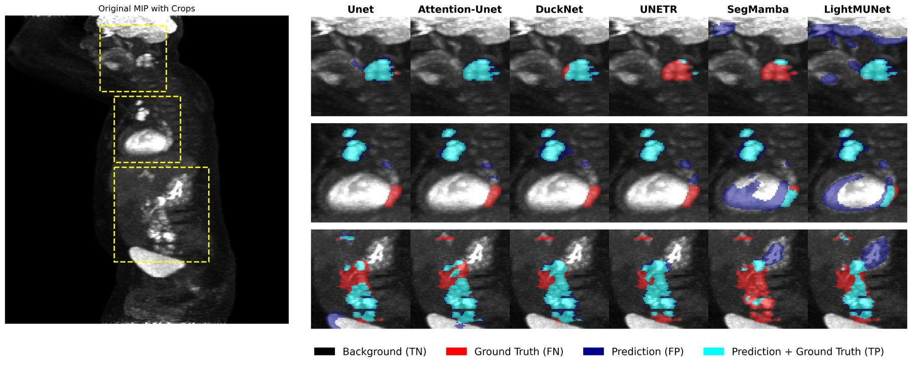
Attention U-Net was the strongest of the CNN architectures we evaluated, and was used for all MIP-based segmentation experiments. The comparison below shows why the choice matters — the transformer and Mamba-based models tend to spill predictions across bright physiological structures.
- Background (TN)
- Ground truth only (FN)
- Prediction only (FP)
- Prediction ∩ ground truth (TP)
Results: classification on 16 MIPs
Segmentation ends in a tie. Classification does not. Using identical CNN encoders with attention pooling and a fully connected head, trained either on 3D volumes or on just 16 MIPs, the projection-based model wins outright on the healthy vs. non-healthy task.
| Metric | 3D dataset | 16 MIPs dataset |
|---|---|---|
| Classification | ||
| Accuracy (%) ↑ | 72.8 ± 3.2 | 80.5 ± 1.7 |
| Precision (%) ↑ | 75.4 ± 6.0 | 83.6 ± 3.3 |
| Recall (%) ↑ | 91.9 ± 8.8 | 89.5 ± 2.9 |
| F1-score (%) ↑ | 82.3 ± 1.2 | 86.4 ± 0.8 |
| Efficiency | ||
| Convergence time (hours) ↓ | 44.7 ± 1.5 | 4.2 ± 0.2 |
| Time per epoch (min) ↓ | 26.1 ± 0.59 | 1.45 ± 0.04 |
| Energy per epoch (Wh) ↓ | 70.7 ± 3.23 | 4.7 ± 0.1 |
The one metric where 3D leads is recall (91.9% vs 89.5%) — but with a standard deviation of 8.8 against 2.9, that lead comes with instability the MIP model does not have. Training is over 10× faster and uses 93.35% less energy per epoch.
How many MIPs?
The number of views is the one free parameter that trades accuracy against cost — it is equivalent to choosing an angular resolution. We trained on sets of 16, 32, 48, 64 and 80 MIPs and tested every model against every configuration.
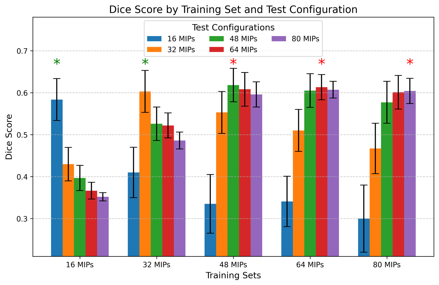
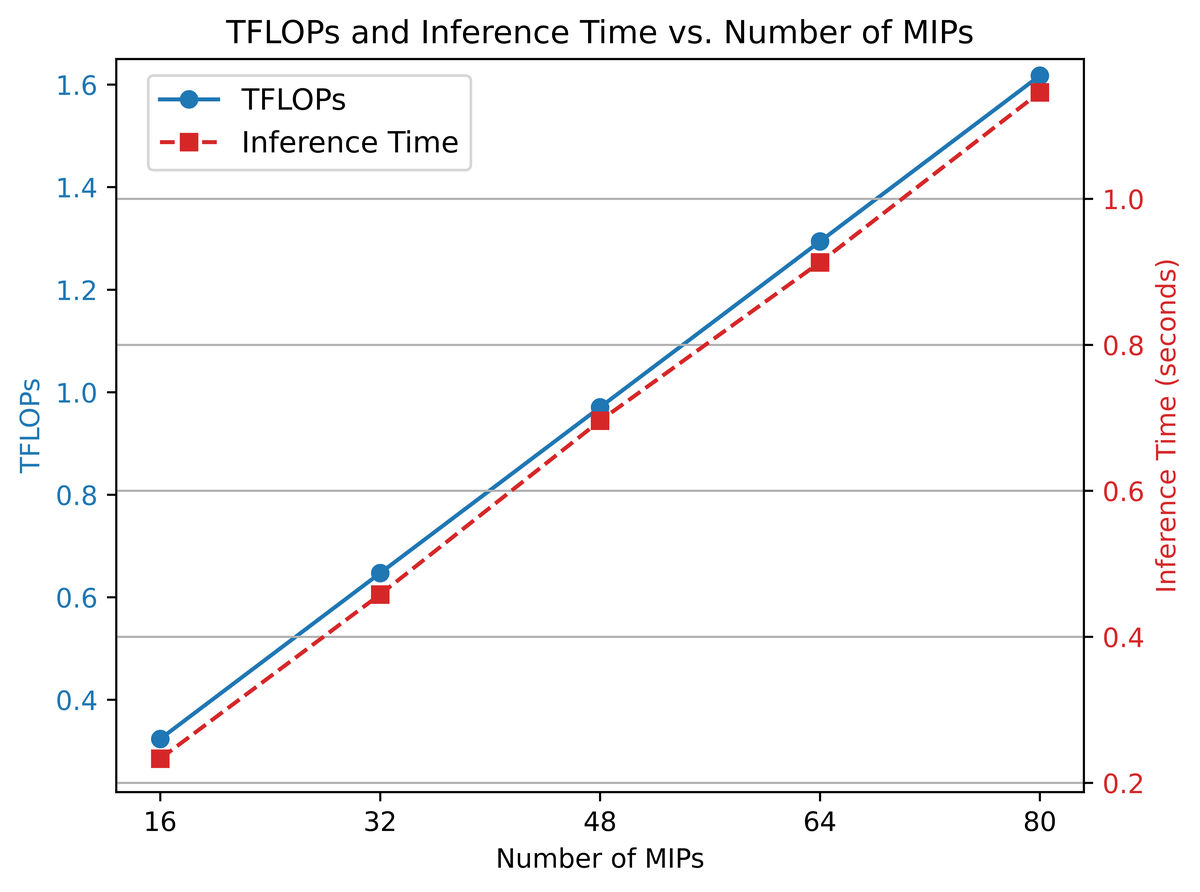
48 MIPs give the highest and most consistent Dice across every train/test combination, and models trained on 48 hold up when tested on 64 or 80 — they are robust to the mismatch, not tuned to one setting. The statistics tell the same story from the other side: the 16- and 32-MIP training sets show a significant gap between their best and second-best test configuration, while 48, 64 and 80 do not, meaning performance has plateaued.
Cost, on the other hand, keeps climbing: both TFLOPs and inference time per case rise steadily with view count. Dice peaks and flattens at 48 while cost does not, which makes 48 the point where more views stop buying accuracy.
Discussion & outlook
Segmenting directly on the projections a radiologist already reads costs nothing in accuracy and saves a great deal of everything else: Dice within 1% of 3D, 26.7% better Hausdorff distance, training time down 55.8–75.8%, energy per epoch down 71.7–76%, and compute down by two orders of magnitude. For classification the projections are simply better, from 16 views alone.
The practical implication is about access rather than leaderboards. A pipeline that trains on a single 24 GB GPU in hours instead of days is one that a hospital research group can actually run, retrain on its own data, and deploy — which matters most exactly where resources are tightest.
Work in progress: bringing CT into the projections by mapping the CT voxels that correspond to each projected PET voxel; building models that exploit structural priors specific to MIPs; and reconstructing 3D annotations from MIP segmentations so the approach can be compared against 3D methods in the volumetric domain too.
Presented at a MICCAI 2025 workshop. Code and preprocessing tools are available in the authors' GitHub repository. This work was supported by a grant from the Tel Aviv University Center for AI and Data Science (TAD).
References
- R. Zarik, N. Kiryati, M. Green, L. Domachevsky, and A. Mayer, "MIP-Based Tumor Segmentation: A Radiologist-Inspired Approach," MICCAI workshop, 2025.
- S. Gatidis, T. Hepp, M. Früh, C. La Fougère, K. Nikolaou, C. Pfannenberg, B. Schölkopf, T. Küstner, C. Cyran, and D. Rubin, "A whole-body FDG-PET/CT dataset with manually annotated tumor lesions," Scientific Data, vol. 9, no. 1, 601, 2022.
- O. Oktay, J. Schlemper, L. L. Folgoc, M. Lee, M. Heinrich, K. Misawa, K. Mori, S. McDonagh, N. Y. Hammerla, B. Kainz, et al., "Attention U-Net: learning where to look for the pancreas," arXiv:1804.03999, 2018.
- L. Heiliger, Z. Marinov, M. Hasin, A. Ferreira, J. Fragemann, K. Pomykala, J. Murray, D. Kersting, V. Alves, R. Stiefelhagen, et al., "autoPET challenge: combining nn-UNet with Swin UNETR augmented by maximum intensity projection classifier," arXiv:2209.01112, 2022.
- A. Hatamizadeh, V. Nath, Y. Tang, D. Yang, H. R. Roth, and D. Xu, "Swin UNETR: Swin Transformers for semantic segmentation of brain tumors in MRI images," MICCAI BrainLes Workshop, pp. 272–284, Springer, 2021.
- M. S. Hofman and R. J. Hicks, "How we read oncologic FDG PET/CT," Cancer Imaging, vol. 16, pp. 1–14, 2016.
- C. S. Constantino, F. P. Oliveira, M. Machado, S. Vinga, and D. C. Costa, "The use of maximum-intensity projections and deep learning adds value to the fully automatic segmentation of lesions avid for [18F]FDG and [68Ga]Ga-PSMA in PET/CT," Journal of Nuclear Medicine, vol. 66, no. 5, pp. 795–801, 2025.
- A. Toosi, S. Harsini, F. Bénard, C. Uribe, and A. Rahmim, "How to segment in 3D using 2D models: automated 3D segmentation of prostate cancer metastatic lesions on PET volumes using multi-angle maximum intensity projections and diffusion models," arXiv:2407.18555, 2024.
- M. Kawakami, K. Hirata, S. Furuya, K. Kobayashi, H. Sugimori, K. Magota, and C. Katoh, "Development of combination methods for detecting malignant uptakes based on physiological uptake detection using object detection with PET-CT MIP images," Frontiers in Medicine, vol. 7, 616746, 2020.
- M. J. Cardoso, W. Li, R. Brown, N. Ma, E. Kerfoot, Y. Wang, B. Murrey, A. Myronenko, C. Zhao, D. Yang, et al., "MONAI: An open-source framework for deep learning in healthcare," arXiv:2211.02701, 2022.